(著者:分析チーム hawai06)
はじめに
ビッグデータや機械学習の技術を活用したDX推進/分析プロジェクトでは、計算量が少なく、機械学習に特有な問題構造を上手く取り扱えるアルゴリズムが必要と考えられる。特に弊社が行なっているようなビジネス課題を解決するプロジェクトの場合は、成果物をビジネスへ活用しやすいよう解釈性に富んでいる方が良く、出力がスパースなアルゴリズムが望ましいと思われる。
一方Frank-Wolfe法とは制約付き最適化問題を解くアルゴリズムであり、最適制御や均衡問題など幅広く用いられている。このアルゴリズムは計算量が少なく、さらに機械学習によく現れる制約条件を取り扱い易いため、近年では機械学習やデータサイエンスなどの分野にも適用されている。また出力される解がスパースになることが知られていることから、このアルゴリズムはビジネス課題の解決手法として候補たり得るものであると思われる。
そこで本稿では、Frank-Wolfe法の詳細およびスパース性が誘導される理由を確認するとともに、実務での有用性を簡易な数値実験を通して確認することとする。
Frank-Wolfe法とは
Frank-Wolfe法は、コンパクトな凸集合$\mathcal{C}$上で定義された、平滑で微分可能な関数$f$の最小値を求めるアルゴリズムである。
解の更新方法は適切なステップ幅を$a_k$を用いて
として記述できる。ステップ幅は$f$の性質により決められる方法が異なり、連続微分可能であるならば直線探索や関数の曲率を用いて定めても良く、また凸であるならば$a_k = \frac{2}{k+2}$としても良い。
$s_k$を求める際は制約付きの線形関数の最小化問題を解くことになるが、制約条件の構造を考慮することで効率良く解ける。例えば$C = \lbrace x | || x|| \le 1 \rbrace$であるならば、Danskin-Bertsekas's Theoremから双対ノルムの劣微分$\partial || \cdot ||_{*}$を用いて$s_k = - \partial || \nabla f(x_k) ||_{*}$となり、計算で求められる場合は簡易に導出できる。$s_k \in \mathcal{C}$より、$x_{k+1}$は常に実行可能解となる。
誘導されるスパース性
初期点$x_0 = 0 \in \mathcal{C}$、$\mathcal{C} \subset \mathbb{R}^n$を仮定すると、Frank-Wolfe法はその解の更新方法より、$x_k$が$\min \lbrace k, n+1 \rbrace$個のデータ点で記述できるため、$k \ll n$の場合はスパース性を持つと言える。このことから$x_k$の非ゼロ要素数はアルゴリズムの収束レートに関連することがわかる。
スパースな解が得られる例として$\mathcal{C} = \lbrace x | || x ||_1 \le 1 \rbrace$を考えると、$\forall k \in \mathbb{N}$に対して$s_k = \text{sign} \left( \nabla f( x^{k-1} )_{i_{k-1}} \right) \cdot e_{i_{k-1}}$となる。よって$k \le n$の場合は$x_k$は非ゼロ要素数が$k$個となり、収束性が良いほどスパースな解が求まり得る。( ただし、$i_{k-1} = \operatorname{argmax}_{i=1,\dots,n} \left| \nabla f( x^{k-1})_{i} \right|$、$e_i$は$i$番目の要素のみ$1$でそれ以外の要素は$0$のベクトル、$\nabla f( x^{k-1})_{i}$は$\nabla f( x^{k-1})$の$i$番目の要素を指す)。
上記より収束性を向上させることでスパースな解を得られる様になるが、アルゴリズムを工夫することでもスパース性は達成され得る。例えば、Fully-Corrective Frank-Wolfe algorithm (以下、FCFW)は次のように解を更新することでFrank-Wolfe法よりもスパースな解が得られるとの報告がある。
初期値$\mathcal{S}_{0} = \lbrace x_0 \rbrace$とする。このアルゴリズムは、これまでの反復で選んだ頂点集合の凸包で最適化計算して解を更新するため、計算量が多くなるという課題がある。
アルゴリズムの比較確認
問題設定
実務でのFrank-Wolfe法の活用を検討するにあたり、機械学習にてよく見られる$l1$-ballを定義域にした次の問題を題材にする。
$x^{*}$は定義域に含まれないよう、定義域の極点をランダムに選んだ$m$点の凸結合に対して$2$倍したものとした。本数値実験では$n$および$m$を適当に変えた場合の、計算時間、出力された解の非ゼロ要素数の個数および$x^{*}$との$l2$-normを確認し、スパース性および解としての適性を評価した。Frank-Wolfe法は解の更新回数により得られる解のスパース度合い変わりうるため、最大更新回数を$10^{6}$と十分多くした。
比較手法
Frank-Wolfe法(以下、FW)、FCFWのスパース性との比較手法として、射影勾配法(以下、PGD)および一般的な方法としてSLSQPを用いた。FWはステップ幅は$\frac{2}{k+2}$および直線探索を別に用いることにし、前者をFW-naive、後者をFW-lineと表記する。PGDは、高次元の問題設定にも適用できるよう、確率単体への射影を基にした射影方法を採用しており、こちらに掲載されているコードをまま使用した。またSLSQPを適用するにあたり、$l1$-ballに対してスラック変数を導入して線形緩和した。これら全ての手法はpythonやそのライブラリを用いて実装している。
結果
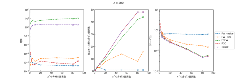
次元数$n = 10^{2}$の場合
$x^{*}$の非ゼロ要素数$m$変化させた時の結果を下に示す。結果の傾向は$n = 10^{2}$と同様になった。計算時間はFCFWが最も長く、SLSQPが次に長いという結果になった。他手法は十分計算時間が短い。$|| x-x^{*} ||_2$はPGDとSLSQPが一致しており、それぞれ最適解に到達していると考えられる。厳密な直線探索をしているFW-lineはFW-naiveと比較して最適解に近い結果が得られた一方、FW-naiveは次元数を増やしても値が減少していない。アルゴリズムの出力解の非ゼロ要素数を確認すると、PGDとSLSQPは$|| x-x^{*} ||_{2}$と同様に一致している。PGDは$x^{*}$の非ゼロ要素数$m$が$1$の場合、本実験においては数値的に不安定になり、原点を出力していたことから$0$の値を示している。FW-naiveは$m \ge 20$以上の場合、出力される解の非ゼロ要素数が$1$となっている。
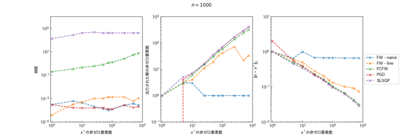
次元数$n = 10^{3}$の場合
先と同様に$m$変化させた時の結果を下に示す。計算時間は、$n = 10^{2}$とは逆にSLSQPが最も長く、FCFWが次に長いという結果となった。他手法は$m$を増加させてもほとんど変わらず、$10^{-3}$秒以下で計算が済んでいる。アルゴリズムの出力解の非ゼロ要素数の傾向は$n = 10^{2}$と同様の結果となったが、縦軸を対数スケールにしているため、上述した$m=1$の時のPGDの値$0$は特異な挙動を示している。
所感
本数値実験において、FCFWは$n \le 10^{3}$においても1秒程度で計算が終了しており、最適解に近く、比較的スパースな解が得られたため、有用な手法であると思われる。しかし、$n = 10^{6}$とした予備実験において$m=10^{2}$では計算時間が3.5時間を超え、$m$を大きくするごとに計算時間が増大していった。内部問題の求解ではできる限り解析的に実装したが、大規模な問題への適用の際はCythonで実装するなど更なる工夫が必要である。
また、PGDとSLSQPは最適解が得られていると考えられる。その中でもPGDは計算時間がかなり短かった。予備実験においても、PGDは最も計算時間が短く$1$秒以内に解が得られた。そのため本問題を実務で取り扱う際は、活躍する可能性が非常に高いと思われる。
FWについては、ステップ幅の決定方法により大きく異なる結果が得られた。FW-naiveは出力される解の非ゼロ要素数が$1$などであり、解の更新がほとんどなされていないことがわかる。最適解が定義域の境界の場合、FW-naiveは収束性が非常に悪くなることが知られており、今回の問題設定はこれに該当する。そのためコスト関数の改善が十分小さすぎるために、解の更新がなされないまま、計算の終了基準を満たしてしまったと考えられる。一方、FW-linearは出力される解の非ゼロ要素数はFW-naiveに次いで小さく、また$|| x-x^{*} ||_{2}$も他手法と比してそれほど大きい値ではない。$|| x-x^{*} ||_{2}$を小さくしたい場合は、スパース性が犠牲になるものの計算の終了基準を厳しくすれば良く、実務では柔軟に利用できると考えられる。
まとめ
本稿では、Frank-Wolfe法は他の手法と比較して、得られる解がスパースになることを解の更新方法および数値実験を通して確認した。数値実験は$l2$ノルムを用いた$l1$-ballへの凸射影を題材にしており、厳密な直線探索を用いたFrank-Wolfe法は計算時間・最適解からの距離の観点から、実用的なスパース解が得られたと思われる。また本稿では実装について述べていないが、実装が比較的容易であった。これらのことから、ビッグデータを取り扱うような実務に際して、Frank-Wolfe法は採用しやすい最適化手法であると言える。
参考文献
- Bertsekas, Dimitri P. Control of uncertain systems with a set-membership description of the uncertainty. Diss. Massachusetts Institute of Technology, 1971.
- Bomze, Immanuel M., Francesco Rinaldi, and Damiano Zeffiro. "Frank–Wolfe and friends: a journey into projection-free first-order optimization methods." 4OR 19 (2021): 313-345.
- Clarkson, Kenneth L. "Coresets, sparse greedy approximation, and the Frank-Wolfe algorithm." ACM Transactions on Algorithms (TALG) 6.4 (2010): 1-30.
- Combettes, Cyrille W., and Sebastian Pokutta. "Revisiting the approximate Carathéodory problem via the Frank-Wolfe algorithm." Mathematical Programming 197.1 (2023): 191-214.
- Duchi, John, et al. "Efficient projections onto the l 1-ball for learning in high dimensions." Proceedings of the 25th international conference on Machine learning. 2008.
- Jaggi, Martin. "Revisiting Frank-Wolfe: Projection-free sparse convex optimization." International conference on machine learning. PMLR, 2013.
- Lacoste-Julien, Simon. "Convergence rate of frank-wolfe for non-convex objectives." arXiv preprint arXiv:1607.00345 (2016).
- Pokutta, Sebastian. "The Frank-Wolfe algorithm: a short introduction." Jahresbericht der Deutschen Mathematiker-Vereinigung 126.1 (2024): 3-35.
参考:使用したコード
以下に本数値実験で使用したコードを掲載する。PGDは、先に述べたようにこちらのコードを用いているため掲載は割愛する。
FW関連(optimization.py)
import numpy as np

def generate_problem(optimal_point : np.array):
    """
    Function Explanation:
        最適解を指定して、コスト関数とその勾配を生成する関数
    Inputs:
        optimal_point : np.array
            最適解
    Returns:
        cost_function : callable
            コスト関数
        grad_cost_function : callable
            コスト関数の勾配
    """

    def cost_function(x : np.array):
        """
        Function Explanation:
            二乗ノルムを用いたコスト関数
        Inputs:
            x : np.array
                点
        Returns:
            (float.)
                関数の値
        """
        return (np.linalg.norm(x - optimal_point, ord=2)**2)/2


    def grad_cost_function(x : np.array):
        """
        Function Explanation:
            二乗ノルムを用いたコスト関数の勾配
        Inputs:
            x : np.array
                点
        Returns:
            (np.array)
                勾配
        """
        return x - optimal_point

    return cost_function, grad_cost_function


def frank_wolfe(x0 : np.array,
                grad_f : callable,
                f      : callable,
                step_size : str,
                max_iter : int = np.inf,
                tol      : float = 1e-6):
    """
    Function Exeplanetion:
        Frank-Wolfe法を用いて、最適化問題を解く関数。
    Inputs:
        x0 : np.array
            初期点
        f : callable
            目的関数
        grad_f : callable
            勾配関数
        step_size : str
            'diminish': 2/2+iteration
            'line search' : 直線探索
        max_iter : int
            最大反復回数
        tol : float
            収束判定の閾値
    Returns:
        x : np.array
            最適解
    """

    # 初期条件の設定
    iteration = 1
    x = x0
    improve = np.inf
    f_list = [f(x0)]

    while (iteration < max_iter) and (improve > tol):
        # 点の設定
        x_k = x
        old = f(x_k)

        # 更新方向
        index = np.argmax(np.abs(grad_f(x)))
        s_k   = np.zeros(len(x))
        s_k[index] =  -np.sign(grad_f(x)[index])
        # ステップ幅
        if step_size == 'diminish':
            step_size = 2/(iteration + 2)
        elif step_size == 'line search':
            norm_s_k = np.linalg.norm(s_k - x, ord=2)
            if  norm_s_k  == 0:
                break
            else:
                step_size = \
                    -np.dot(s_k, grad_f(x)) / norm_s_k**2
            if step_size < 0:
                step_size = 0
            elif step_size > 1:
                step_size = 1
        # 更新
        print(iteration)
        x = x_k + step_size * (s_k - x_k)
        iteration += 1
        improve = 1 - (f(x) / old )
        f_list.append(f(x))

    return x#, f_list


def find(s, S):
    for i in range(len(S)):
        if np.all(S[i] == s):
            return True
    return False

def FullyCorrectiveFrankWolfe(x0 : np.array,
                              grad_f : callable,
                              f      : callable,
                              optimal_point : np.array,
                              max_iter : int = np.inf,
                              tol      : float = 1e-6,
                              inner_max_iter : int = np.inf,
                              inner_tol : float = 1e-6):

    """
    Function Explanation:
        Fully Corrective Frank-Wolfe法を用いて、最適化問題を解く関数。
    Inputs:
        x0 : np.array
            初期点
        f : callable
            目的関数
        grad_f : callable
            勾配関数
        max_iter : int
            最大反復回数
        tol : float
            収束判定の閾値
        optimal_point : np.array
            本数値実験の最適解
        inner_max_iter : int
            内部問題の最大反復回数
        inner_tol : float
            内部問題の収束判定の閾値
    Returns:
        x : np.array
            最適解
    """

    # 初期条件の設定
    iteration = 1
    x = x0
    S = list()
    S.append(x)
    impove = np.inf
    f_list = [f(x0)]

    while (iteration < max_iter) and (impove > tol):
        # 点の設定
        x_k = x
        old = f(x_k)

        # Sの集合を構築
        ## 要素取得
        index = np.argmax(np.abs(grad_f(x_k)))
        s_k   = np.zeros(len(x_k))
        s_k[index] =  -np.sign(grad_f(x_k)[index])
        ## 要素の追加
        if find(s_k, S) == False:
            S.append(s_k)


        # 内部問題を解いて解の更新
        inner_improve   = np.inf
        inner_iteration = 1
        while (inner_iteration < inner_max_iter) and (inner_improve > inner_tol):
            # ループ情報の設定
            inner_old = f(x)
            inner_iteration += 1

            # 内部問題の求解
            inner_index = np.argmin(np.dot(np.array(S), grad_f(x)))
            norm_s_k = np.linalg.norm(S[inner_index] - x, ord=2)
            if  norm_s_k  == 0:
                break
            else:
                step_size = \
                    -np.dot(S[inner_index],grad_f(x)) / norm_s_k**2
            if step_size < 0:
                step_size = 0
            elif step_size > 1:
                step_size = 1
            x =  x + step_size * (S[inner_index] - x)


            # ループ情報の更新

            inner_improve = 1 - (f(x) / inner_old )


        # ループ情報の更新
        iteration += 1
        improve = 1 - (f(x) / old )
        f_list.append(f(x))

    return x#, f_list

if __name__ == "__main__":
    # ライブラリの読み込み
    import os
    from problem_setting import generate_optimal_point


    # 最適解の生成
    dimensions = 100
    combination_num = 10
    optimal_point = generate_optimal_point(dimensions,
                                           combination_num,
                                           in_range = 'out',
                                           out_coef = 2)
    # 問題の生成
    f, grad_f = generate_problem(optimal_point)

    # 最適化アルゴリズムの実行
    initial_point = np.zeros(dimensions)
    print("FW")
    FW_solution = frank_wolfe(initial_point,
                              grad_f, f,
                              step_size = 'diminish',
                              max_iter = 10000, tol = 1e-6)
    print("FC")
    FCFW_solution = FullyCorrectiveFrankWolfe(
        initial_point,
        grad_f, f,
        optimal_point,
        max_iter = 1000, tol = 1e-6,
        inner_max_iter = 1000, inner_tol = 1e-6)
SLSQP(slsqp.py)
import numpy as np
from problem_setting import generate_optimal_point
from optimization import generate_problem
from scipy.optimize import minimize
import os
import copy


class SLSQP:

    def __init__(self,
                 optimal_point : np.array,
                 dimensions    : np.array,
                 initial_point : np.array):

        self.dimensions    = dimensions
        self.optimal_point = optimal_point
        self.initial_point = self._generate_initial_point_for_slack_var(
            initial_point
            )

    def _generate_initial_point_for_slack_var(self,
                                              optimal_point : np.array):
        copy_optimal_point          = np.copy(optimal_point)
        initial_point_for_slack_var = np.concatenate(
            [optimal_point, copy_optimal_point], 0
            )
        return initial_point_for_slack_var

    def _upper_bound_const(self, index):
        return {'type': 'ineq',
                'fun' : lambda x:  x[index + self.dimensions] - x[index]}

    def _genrate_upper_bound_const(self):
        const_list = list()
        for index in range(self.dimensions):
            const_list.append(self._upper_bound_const(index))
        return const_list

    def _lower_bound_const(self, index):
        return {'type': 'ineq',
                'fun' : lambda x:  x[index] + x[index + self.dimensions]}

    def _genrate_lower_bound_const(self):
        const_list = list()
        for index in range(self.dimensions):
            const_list.append(self._lower_bound_const(index))
        return const_list


    def _genrate_l1_bound_const(self):
        const_list = list()
        const_list.append(
            {'type': 'ineq',
             'fun' : lambda x:  1- np.sum(x[self.dimensions:])}
            )
        return const_list

    def _generate_cost_function(self):
        """
        Function Explanation:
            二乗ノルムを用いたコスト関数
        Inputs:
            x : np.array
                点
        Returns:
            (float.)
            関数の値
        """
        return lambda x: np.sum(x[self.dimensions:]**2)/2 - \
                         np.dot(x[:self.dimensions], self.optimal_point) + \
                         np.sum(self.optimal_point**2)/2

    def solve(self):
        # 問題の生成
        cost_function  = self._generate_cost_function()

        # 制約条件の作成
        ## l1-ball
        constraints = []
        constraints.extend(self._genrate_upper_bound_const())
        constraints.extend(self._genrate_lower_bound_const())
        constraints.extend(self._genrate_l1_bound_const())
        ## box_const
        bounds = []
        bounds.extend([(-1, 1) for i in range(self.dimensions)])
        bounds.extend([(0, 1) for i in range(self.dimensions)])


        solution = minimize(
            cost_function, x0 = self.initial_point,
            method = 'SLSQP',
            constraints = constraints,
            bounds = bounds,
            options = {'maxiter' :1000 , 'disp' : True},
            tol = 1e-9
            )
        return solution

    def solution_arrange(self,
                         solution, eps = 1e-6):

        solution_mask =  np.abs(
            solution.x[:self.dimensions]
            ) >  eps
        optimal_solution      = np.empty(self.dimensions)
        optimal_solution[solution_mask]  = solution.x[:self.dimensions][solution_mask]
        optimal_solution[~solution_mask] = np.zeros(self.dimensions)[~solution_mask]

        return optimal_solution


if __name__ == "__main__":

    # 最適解の生成
    dimensions = 10
    combination_num = 2
    optimal_point = generate_optimal_point(dimensions,
                                           combination_num,
                                           in_range = 'in',
                                           out_coef = 2)
    #optimal_point = np.random.randn(dimensions)
    #optimal_point = optimal_point / np.sum(np.abs(optimal_point))

    initial_point = np.zeros(dimensions)

    # 問題の生成

    func = SLSQP(optimal_point,
                 dimensions,
                 initial_point)
    func.initial_point.shape
    solution = func.solve()
    optimal_solution = func.solution_arrange(solution)

    print(optimal_solution)
    print(optimal_point)
最適解の生成(problem_setting.py)
import numpy as np


def generate_optimal_point(dimensions : int,
                           combination_num      : int,
                           in_range   : str,
                           out_coef : float = 1.0):
    """
    Function Explanation:
        l1-ball上の極点の凸結合として定義される、スパースな点を生成する関数。
        'in_range'を変更することで、生成される点がl1-ballの内外のどちらになるかを指定できる。
    Inputs:
        dimensions : int
            初期点の次元数
        combination_num : int
            初期点の生成にあたり、利用する極点の数
            (注意:combination_num <= dimensions)
        in_range : str
            生成される点がl1-ballの内外のどちらになるかを指定するパラメータ
            'in' : l1-ballの内部に生成される
            'out' : l1-ballの外部に生成される
        out_coef : float
            'in_range'が'out'の場合に、l1-ballの外部に生成される点の係数
    Returns:
        coordinates : np.array
            生成された点
    """
    # スパースな点が生成されるかの確認
    if combination_num > dimensions:
        raise ValueError("'combination_num' must be less than or equal to 'dimensions'.")

    # 初期点生成にあたり、関与する座標の決定
    # 各要素が0からdimensions-1までの整数値のベクトル
    rng = np.random.default_rng()
    coordinates_list = rng.integers(low = 0, high = dimensions,
                                    size= combination_num, dtype=np.int64, endpoint=True)

    # 初期生成のための重み作成
    weights = rng.uniform(low=-1, high=1, size=combination_num)
    weights = weights / np.sum(np.abs(weights))


    # 初期点生成
    coordinates = np.zeros(dimensions)
    for i, index in enumerate(coordinates_list):
         coordinates[index] += weights[i]

    # l1-ballの外部に生成される場合
    if in_range == 'out':
        coordinates = coordinates * out_coef
    elif in_range == 'in':
        pass
    else:
        raise ValueError("in_range must be 'in' or 'out'.")

    return coordinates
数値実験(experiment.py)
import os
import pickle
import numpy as np
import pandas as pd
import matplotlib.pyplot as plt
from time import time
plt.rcParams['font.family'] = 'Hiragino Sans'
plt.rcParams['xtick.direction'] = 'in'
plt.rcParams['ytick.direction'] = 'in'

# 問題設定のライブラリ
from problem_setting import generate_optimal_point
# frank-wolfe法のライブラリ
from optimization import frank_wolfe, FullyCorrectiveFrankWolfe,generate_problem
# SLSQPのライブラリ
from slsqp import SLSQP
# PGDのライブラリ
from pgd import euclidean_proj_l1ball


# 実験の初期点を保存関数(確率的にエラーが出るため、保存)
##################################################
def save_optimal_point(dimensions       : int,
                       non_zero_nums    : dict,
                       in_range         : str,
                       out_coef         : int,
                       save_name        : str):
    # 格納箱
    dim_optimal_dict = {num : None for num in non_zero_nums}

    # データ点の生成
    for num in non_zero_nums:
        optimal_point = generate_optimal_point(
            dimensions,
            combination_num = num,
            in_range = in_range, out_coef = out_coef
            )
        dim_optimal_dict[num] = optimal_point
    # データ保存
    with open(save_name, "wb") as f:
        pickle.dump(dim_optimal_dict, f)

    return None
##################################################


# 実験の初期設定の準備
## 準備
problem_setting_dict = {
    100   : {'non_zero_nums' : [1, 5, 10, 20, 50, 80, 90],
             'method_names'  : ['FW - naive', 'FW - line', 'FCFW', 'PGD', 'SLSQP'],
             'save_name'     : 'dim_100_optimal_dict.pkl',
             'solution_save_name' : 'dim_100_solution_dict.pkl',
             'time_save_name' : 'dim_100_time_dict.pkl'},


    10**6 : {'non_zero_nums' : [1, 5, 10, 50, 100, 500, 1000, 10000],
             'method_names'  : ['FW - naive', 'FW - line', 'FCFW', 'PGD'],
             'save_name'     : 'dim_10**6_optimal_dict.pkl',
             'solution_save_name' : 'dim_10**6_solution_dict.pkl',
             'time_save_name' : 'dim_10**6_time_dict.pkl'},

    1000  : {'non_zero_nums' : [1, 5, 10, 25, 50, 75 ,100, 250, 500, 750],
             'method_names'  : ['FW - naive', 'FW - line', 'FCFW', 'PGD', 'SLSQP'],
             'save_name'     : 'dim_1000_optimal_dict.pkl',
             'solution_save_name' : 'dim_1000_solution_dict.pkl',
             'time_save_name' : 'dim_1000_time_dict.pkl'},
    }

## データ点生成+保存
#dimensions = 100
#dimensions = 10**6
#dimensions = 1000
#save_optimal_point(
#    dimensions,
#    problem_setting_dict[dimensions]['non_zero_nums'],
#    in_range = 'out',
#    out_coef = 2,
#    save_name = problem_setting_dict[dimensions]['save_name']
#    )


# 問題を解く
## 初期設定
dimensions = 1000
## 問題の読み込み
with open(problem_setting_dict[dimensions]['save_name'], 'rb') as f:
    dim_optimal_dict = pickle.load(f)
# 各手法の計算
## 計算結果の格納箱
solution_dict = {
    method : {num : None
              for num in problem_setting_dict[dimensions]['non_zero_nums']}
    for method in problem_setting_dict[dimensions]['method_names']
    }
time_dict  = {
    method : {num : None
              for num in problem_setting_dict[dimensions]['non_zero_nums']}
    for method in problem_setting_dict[dimensions]['method_names']
    }
## 計算
for num in problem_setting_dict[dimensions]['non_zero_nums']:
    # 初期設定
    ## 最適解
    optimal_point = dim_optimal_dict[num]


    # FC、FCFW
    ## 問題、初期点の生成
    f, grad_f = generate_problem(optimal_point)
    initial_point = np.zeros(dimensions)
    ## 実行
    ### FW diminish
    print('num:', num, ' FW - naiveを開始')
    FW_naive_start = time()
    solution_dict['FW - naive'][num] = frank_wolfe(
        initial_point, grad_f, f,step_size = 'diminish',
        max_iter = 10000, tol = 1e-6
        )
    FW_naive_end  = time()
    time_dict['FW - naive'][num] = FW_naive_end - FW_naive_start
    print('num:', num, ' FW - naiveの時間:', time_dict['FW - naive'][num])

    ### FW 直線探索
    print('num:', num, 'FW - lineを開始')
    FW_line_start = time()
    solution_dict['FW - line'][num] = frank_wolfe(
        initial_point, grad_f, f,step_size = 'line search',
        max_iter = 10000, tol = 1e-6
        )
    FW_line_end  = time()
    time_dict['FW - line'][num] = FW_line_end - FW_line_start
    print('num:', num, ' FW - lineの時間:', time_dict['FW - line'][num])


    ### FCFW
    print('num:', num, 'FCFWを開始')
    FCFW_start = time()
    solution_dict['FCFW'][num] = FullyCorrectiveFrankWolfe(
        initial_point, grad_f, f,
        optimal_point,
        max_iter = 10000    , tol = 1e-6,
        inner_max_iter = 1000, inner_tol = 1e-6
        )
    FCFW_end  = time()
    time_dict['FCFW'][num] = FCFW_end - FCFW_start
    print('num:', num, ' FCFWの時間:', time_dict['FCFW'][num])


    # PGD
    print('num:', num, 'PGDを開始')
    PGD_start = time()
    solution_dict['PGD'][num] = euclidean_proj_l1ball(
        optimal_point, s=1
        )
    PGD_end  = time()
    time_dict['PGD'][num] = PGD_end - PGD_start
    print('num:', num, ' PGDの時間:', time_dict['PGD'][num])


    # SLSQP(次元数100、1000の時だけ実行)
    if (dimensions == 100) | (dimensions == 1000):
        print('num:', num, 'SLSQPを開始')
        SLSQP_start = time()
        # 初期設定
        func = SLSQP(optimal_point,
                     dimensions,
                     initial_point)
        # 求解
        slsqp_solution = func.solve()
        # 解の整形
        solution_dict['SLSQP'][num] = func.solution_arrange(slsqp_solution)
        SLSQP_end  = time()
        time_dict['SLSQP'][num] = SLSQP_end - SLSQP_start
        print('num:', num, ' SLSQPの時間:', time_dict['SLSQP'][num])


# 結果の保存
with open(problem_setting_dict[dimensions]['solution_save_name'],
          "wb") as f:
    pickle.dump(solution_dict, f)

with open(problem_setting_dict[dimensions]['time_save_name'],
          "wb") as f:
    pickle.dump(time_dict, f)


# 結果を開く
dimensions =100
with open(problem_setting_dict[dimensions]['save_name'], 'rb') as f:
    dim_optimal_dict = pickle.load(f)
with open(problem_setting_dict[dimensions]['solution_save_name'], 'rb') as f:
    solution_dict  = pickle.load(f)
with open(problem_setting_dict[dimensions]['time_save_name'], 'rb') as f:
    time_dict = pickle.load(f)


# 可視化
#################################################
plt.figure(figsize = (30, 5))
if dimensions == 100:
    plt.suptitle('$n=100$')
elif dimensions == 1000:
    plt.suptitle('$n=1000$')

plt.subplot(1,3,1)
for method in problem_setting_dict[dimensions]['method_names']:
    plt.plot(problem_setting_dict[dimensions]['non_zero_nums'],
             [time_dict[method][num]
              for num in problem_setting_dict[dimensions]['non_zero_nums']],
             'x--', label = method)
    plt.xlabel('$x^*$の非ゼロ要素数')
    plt.ylabel('時間')
if dimensions == 100:
    plt.xlim([0,100])
    plt.xticks([20 * i for i in range(6)])
    plt.ylim([1e-5,100])
    plt.yscale('log')
elif dimensions == 1000:
    plt.xlim([0.9,1000])
    plt.ylim([1e-5,10e3])
    plt.xscale('log')
    plt.yscale('log')


plt.subplot(1,3,2)
for method in problem_setting_dict[dimensions]['method_names']:
    plt.plot(problem_setting_dict[dimensions]['non_zero_nums'],
             [np.sum(np.abs(solution_dict[method][num]) > 1e-6)
              for num in problem_setting_dict[dimensions]['non_zero_nums']],
             'x--', label = method)
    plt.xlabel('$x^*$の非ゼロ要素数')
    plt.ylabel('出力された解の非ゼロ要素数')
if dimensions == 100:
    plt.xlim([0,100])
    plt.xticks([20 * i for i in range(6)])
    plt.ylim([0,50])
    plt.yticks([10 * i for i in range(6)])
elif dimensions == 1000:
    plt.xlim([0.9,1000])
    plt.ylim([0.1,1000])
    plt.xscale('log')
    plt.yscale('log')


plt.subplot(1,3,3)
for method in problem_setting_dict[dimensions]['method_names']:

    plt.plot(problem_setting_dict[dimensions]['non_zero_nums'],
             [np.linalg.norm(
                 solution_dict[method][num] - dim_optimal_dict[num],
                 ord = 2
                 )
              for num in problem_setting_dict[dimensions]['non_zero_nums']],
             'x--', label = method)
    plt.xlabel('$x^*$の非ゼロ要素数')
    plt.ylabel('$\| x -x^* \|_2$')
    plt.legend(loc='center left', bbox_to_anchor=(1, 0.5))

if dimensions == 100:
    plt.xlim([0,100])
    plt.xticks([20 * i for i in range(6)])
    plt.yscale('log')
    plt.ylim([0.01,10])
elif dimensions == 1000:
    plt.xlim([0.9,1000])
    plt.ylim([1e-2,10])
    plt.xscale('log')
    plt.yscale('log')

plt.show()
#################################################